Alternate grid background color in excel when a value of a single column changes?

Question

I need a formula for conditional formatting to make an Excel 2010 spreadsheet alternate highlighting when a single column changes. This question, "How can I alternate grid background color in excel when a value of a single column changes?", is exactly what I want to do, but the suggested solution didn't work for me--it just highlights the first row of each matching value.

I know how to use conditional formatting, but for the life of me I can't figure out or find any pointers on the net so far to make this work. Ideas?

Here is a link to a picture of how I want my spreadsheet to look when I'm done. Basically I want every other Disp Number value row to be highlighted. Seems like it would be a common thing to want to do, and I've seen this asked for in various places, but people struggle with making it work.

Picture of desired end result

Answer 1

This answer is copied straight from stackoverflow.com Alternating coloring groups of rows in Excel.

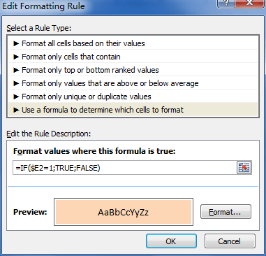
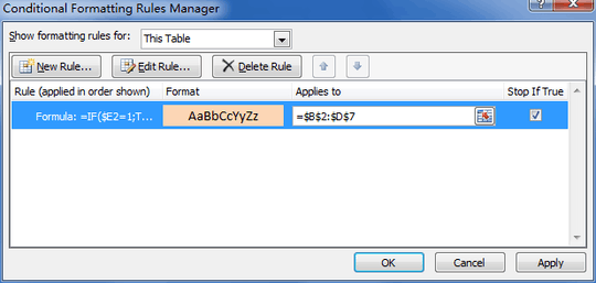
I use this formula to get the input for a conditional formatting:

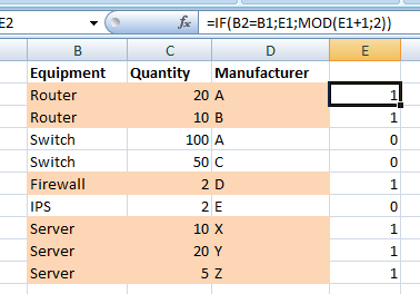
=IF(B2=B1,E1,MOD(E1+1,2))    [content of cell E2]

Where column B contains the item that needs to be grouped and E is an auxiliary column. Every time that the upper cell (B1 on this case) is the same as the current one (B2), the upper row content from column E is returned. Otherwise, it will return that content plus 1 MOD 2 (that is, the outupt will be 0 or 1, depending on the value of the upper cell).

As an alternative to the MOD function, you could use 1 - E1. So full formula is =IF(B2=B1,E1,1-E1).

A pretty similar method is described in Color Banding Based On Content, where a downloadable example is included.

Answer 2

This is a whole lot simpler if you’re willing to create a couple of helper columns.  For example, set Y2 to =($A2=$A1), set Z1 to TRUE, set Z2 to =IF($Y2, $Z1, NOT($Z1)), and drag/fill Y2:Z2 down to the last row where you have data.  Column Z will alternate between TRUE and FALSE in the manner that you desire.  Of course you can hide columns Y and Z when you’ve gotten it debugged.

In case this isn’t clear: the cell in column Y determines whether the values of A on this row and the preceding one are the same, so it is FALSE on the first row of each new value and then TRUE throughout the rest of the block.  And column Z is a chain of dominos –– each value depends on the one above it.  If the value in column Y is TRUE, Z keeps the same value as the row above; otherwise, Z switches.

Answer 3

The helper column alternating 1 and 0 does not need a MOD() function. A simple formula for E2 is -

=IF(B2=B1,E1,1-E1)