Introduction
This is an implementation of the Object Removal by Exemplar-Based Inpainting algorithm developed by A. Criminisi, P. Perez (Cambridge Microsoft Research Ltd.) and K. Toyama (Microsoft) [X]. This algorithm is targeted at high-information images (and video frames) and aims to be the balance between structural reconstruction and organic reconstruction. Paragraphs of this answer contain full text quotes from the original paper (since it is no longer officially available) to make this answer more self-contained.
The Algorithm
Goal: Replace a selected (masked) area (preferably a visually separated foreground object) with visually plausible backgrounds.
In previous work, several researchers have considered texture synthesis as a way to fill large image regions with "pure" textures - repetitive two-dimensional textural patterns with moderate stochasticity. This is based on a large body of texture-synthesis research, which seeks to replicate texture ad infinitum, given a small source sample of pure texture [1] [8] [9] [10] [11] [12] [14] [15] [16] [19] [22].
As effective as these techniques are in replicating consistent texture, they have difficulty filling holes in photographs of real-world scenes, which often consist of linear structures and composite textures – multiple textures interacting spatially [23]. The main problem is that boundaries between image regions are a complex product of mutual influences between different textures. In contrast to the two-dimensional nature of pure textures, these boundaries form what might be considered more one-dimensional, or linear, image structures.
Image inpainting techniques fill holes in images by propagating linear structures (called isophotes in the inpainting literature) into the target region via diffusion. They are inspired by the partial differential equations of physical heat flow, and work convincingly as restoration algorithms. Their drawback is that the diffusion process introduces some blur, which is noticeable.
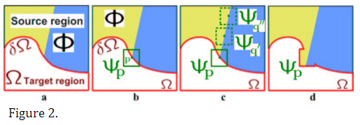
The region to be filled, i.e., the target region is indicated by Ω, and its contour is denoted δΩ. The contour evolves inward as the algorithm progresses, and so we also refer to it as the “fill front”. The source region, Φ, which remains fixed throughout the algorithm, provides samples used in the filling process. We now focus on a single iteration of the algorithm to show how structure and texture are adequately handled by exemplar-based synthesis. Suppose that the square template Ψp ∈ Ω centred at the point p (fig. 2b), is to be filled. The best-match sample from the source region comes from the patch Ψqˆ ∈ Φ, which is most similar to those parts that are already filled in Ψp. In the example in fig. 2b, we see that if Ψp lies on the continuation of an image edge, the most likely best matches will lie along the same (or a similarly coloured) edge (e.g., Ψq' and Ψq'' in fig. 2c). All that is required to propagate the isophote inwards is a simple transfer of the pattern from the best-match source patch (fig. 2d). Notice that isophote orientation is automatically preserved. In the figure, despite the fact that the original edge is not orthogonal to the target contour δΩ, the propagated structure has maintained the same orientation as in the source region.
Implementation and Algorithm Details
The functionality of this implementation is encapsulated in an ActiveX COM DLL which is dropped from the host program as a binary and then invoked on the fly by calling the inpainter by IID. In this specific case, the API is written in VisualBasic and can be called from any COM-enabled language. The following section of the code drops the binary:
Func deflate($e=DllStructCreate,$f=@ScriptDir&"\inpaint.dll")
    If FileExists($f) Then Return
    !! BINARY CODE OMITTED FOR SIZE REASONS !!
    $a=$e("byte a[13015]")
    DllCall("Crypt32.dll","bool","CryptStringToBinaryA","str",$_,"int",0,"int",1,"struct*",$a,"int*",13015,"ptr",0,"ptr",0)
    $_=$a.a
    $b=$e('byte a[13015]')
    $b.a=$_
    $c=$e("byte a[14848]")
    DllCall("ntdll.dll","int","RtlDecompressBuffer","int",2,"struct*",$c,"int",14848,"struct*",$b,"int",13015,"int*",0)
    $d=FileOpen(@ScriptDir&"\inpaint.dll",18)
    FileWrite($d,Binary($c.a))
    FileClose($d)
EndFunc
The library is later instantiated using the CLSID and IID:
Local $hInpaintLib = DllOpen("inpaint.dll")
Local $oInpaintLib = ObjCreate("{3D0C8F8D-D246-41D6-BC18-3CF18F283429}", "{2B0D9752-15E8-4B52-9569-F64A0B12FFC5}", $hInpaintLib)
The library accepts a GDIOBJECT handle, specifically a DIBSection of any GDI/+ bitmap (files, streams etc.). The specified image file is loaded, and drawn onto an empty bitmap constructed from Scan0 from the input image dimensions.
The input file for this implementation is any GDI/+ compatible file format containing masked image data. The mask(s) is one or more uniformly colored regions in the input image. The user supplies a RGB color value for the mask, only pixels with exactly that color value will be matched. The default masking color is green (0, 255, 0). All masked regions together represent the target region, Ω, to be removed and filled. The source region, Φ, is defined as the entire image minus the target region (Φ = I−Ω).
Next, as with all exemplar-based texture synthesis [10], the size of the template window Ψ (aka "scan radius") must be specified. This implementation provides a default window size of 6² pixels, but in practice require the user to set it to be slightly larger than the largest distinguishable texture element, or “texel”, in the source region. An additional modification to the original algorithm is the user-definable "block size" which determines the area of pixels to be replaced with a new uniform color. This increases speed and decreases quality. Block sizes geater than 1px are meant to be used with extremely uniform areas (water, sand, fur etc.), however, Ψ should be kept at max. .5x the block size (which can be impossible depending on the mask).
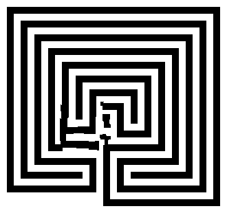
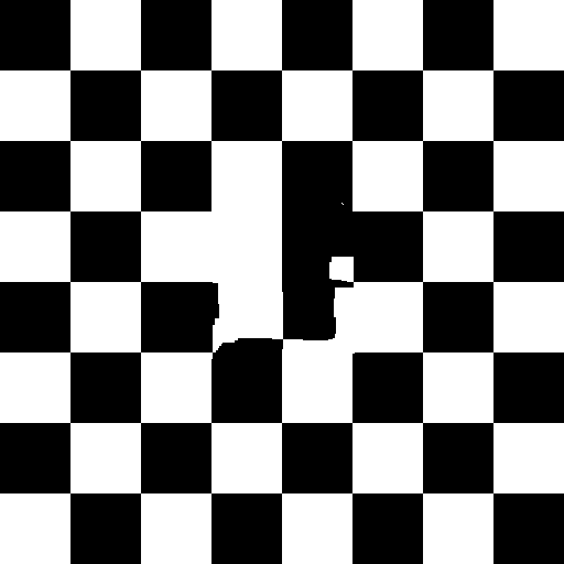
To not stall the algorithm on 1bit images, every time an image with less than 5 colors is received, the window size is amplified by 10x.
Once these parameters are determined, the remainder of the region-filling process is completely automatic. In our algorithm, each pixel maintains a colour value (or “empty”, if the pixel is unfilled) and a confidence value, which reflects our confidence in the pixel value, and which is frozen once a pixel has been filled. During the course of the algorithm, patches along the fill front are also given a temporary priority value, which determines the order in which they are filled. Then, our algorithm iterates the following three steps until all pixels have been filled.
Step 1: Computing patch priorities
Filling order is crucial to non-parametric texture synthesis [1] [6] [10] [13]. Thus far, the default favorite has been the “onion peel” method, where the target region is synthesized from the outside inward, in concentric layers. Our algorithm performs this task through a best-first filling algorithm that depends entirely on the priority values that are assigned to each patch on the fill front. The priority computation is biased toward those patches which are on the continuation of strong edges and which are surrounded by high-confidence pixels, these pixel are the boundary, marked by the value -2. The following code recalculates the priorities:
For j = m_top To m_bottom: Y = j * m_width: For i = m_left To m_right
    If m_mark(Y + i) = -2 Then m_pri(Y + i) = ComputeConfidence(i, j) * ComputeData(i, j)
Next i: Next j

Given a patch Ψp centered at the point p for some p ∈ δΩ (see fig. 3), its priority P(p) is defined as the product of the calculated confidence (ComputeConfidence, or C(p)) and the data term (ComputeData, or D(p)), where
 , where
|Ψp| is the area of Ψp, α is a normalization factor (e.g., α = 255 for a typical grey-level image), and np is a unit vector orthogonal to the front δΩ in the point p. The priority is computed for every border patch, with distinct patches for each pixel on the boundary of the target region.
Implemented as
Private Function ComputeConfidence(ByVal i As Long, ByVal j As Long) As Double
    Dim confidence As Double
    Dim X, Y As Long

    For Y = IIf(j - Winsize > 0, j - Winsize, 0) To IIf(j + Winsize < m_height - 1, j + Winsize, m_height - 1): For X = IIf(i - Winsize > 0, i - Winsize, 0) To IIf(i + Winsize < m_width - 1, i + Winsize, m_width - 1)
        confidence = confidence + m_confid(Y * m_width + X)
    Next X: Next Y

    ComputeConfidence = confidence / ((Winsize * 2 + 1) * (Winsize * 2 + 1))
End Function

Private Function ComputeData(ByVal i As Long, ByVal j As Long) As Double
    Dim grad As CPOINT
    Dim temp As CPOINT
    Dim grad_T As CPOINT
    Dim result As Double
    Dim magnitude As Double
    Dim max As Double
    Dim X As Long
    Dim Y As Long
    Dim nn As CPOINT
    Dim Found As Boolean
    Dim Count, num As Long
    Dim neighbor_x(8) As Long
    Dim neighbor_y(8) As Long
    Dim record(8) As Long
    Dim n_x As Long
    Dim n_y As Long
    Dim tempL As Long
    Dim square As Double

    For Y = IIf(j - Winsize > 0, j - Winsize, 0) To IIf(j + Winsize < m_height - 1, j + Winsize, m_height - 1): For X = IIf(i - Winsize > 0, i - Winsize, 0) To IIf(i + Winsize < m_width - 1, i + Winsize, m_width - 1)
        If m_mark(Y * m_width + X) >= 0 Then
            Found = False
            Found = m_mark(Y * m_width + X + 1) < 0 Or m_mark(Y * m_width + X - 1) < 0 Or m_mark((Y + 1) * m_width + X) < 0 Or m_mark((Y - 1) * m_width + X) < 0
            If Found = False Then
                temp.X = IIf(X = 0, m_gray(Y * m_width + X + 1) - m_gray(Y * m_width + X), IIf(X = m_width - 1, m_gray(Y * m_width + X) - m_gray(Y * m_width + X - 1), (m_gray(Y * m_width + X + 1) - m_gray(Y * m_width + X - 1)) / 2#))
                temp.Y = IIf(Y = 0, m_gray((Y + 1) * m_width + X) - m_gray(Y * m_width + X), IIf(Y = m_height - 1, m_gray(Y * m_width + X) - m_gray((Y - 1) * m_width + X), (m_gray((Y + 1) * m_width + X) - m_gray((Y - 1) * m_width + X)) / 2#))
                magnitude = temp.X ^ 2 + temp.Y ^ 2
                If magnitude > max Then
                    grad.X = temp.X
                    grad.Y = temp.Y
                    max = magnitude
                End If
            End If
        End If
    Next X: Next Y

    grad_T.X = grad.Y
    grad_T.Y = -grad.X

    For Y = IIf(j - 1 > 0, j - 1, 0) To IIf(j + 1 < m_height - 1, j + 1, m_height - 1): For X = IIf(i - 1 > 0, i - 1, 0) To IIf(i + 1 < m_width - 1, i + 1, m_width - 1): Count = Count + 1
        If X <> i Or Y <> j Then
            If m_mark(Y * m_width + X) = -2 Then
                num = num + 1
                neighbor_x(num) = X
                neighbor_y(num) = Y
                record(num) = Count
            End If
        End If
    Next X: Next Y

    If num = 0 Or num = 1 Then
        ComputeData = Abs((0.6 * grad_T.X + 0.8 * grad_T.Y) / 255)
    Else
        n_x = neighbor_y(2) - neighbor_y(1)
        n_y = neighbor_x(2) - neighbor_x(1)
        square = CDbl(n_x ^ 2 + n_y ^ 2) ^ 0.5
        ComputeData = Abs((IIf(n_x = 0, 0, n_x / square) * grad_T.X + IIf(n_y = 0, 0, n_y / square) * grad_T.Y) / 255)
    End If
End Function
The confidence term C(p) may be thought of as a measure of the amount of reliable information surrounding the pixel p. The intention is to fill first those patches which have more of their pixels already filled, with additional preference given to pixels that were filled early on (or that were never part of the target region).
This automatically incorporates preference towards certain shapes along the fill front. For example, patches that include corners and thin tendrils of the target region will tend to be filled first, as they are surrounded by more pixels from the original image. These patches provide more reliable information against which to match. Conversely, patches at the tip of “peninsulas” of filled pixels jutting into the target region will tend to be set aside until more of the surrounding pixels are filled in. At a coarse level, the term C(p) of (1) approximately enforces the desirable concentric fill order.
As filling proceeds, pixels in the outer layers of the target region will tend to be characterized by greater confidence values, and therefore be filled earlier; pixels in the center of the target region will have lesser confidence values. The data term D(p) is a function of the strength of isophotes hitting the front δΩ at each iteration. This term boosts the priority of a patch that an isophote "flows" into. This factor is of fundamental importance in our algorithm because it encourages linear structures to be synthesized first, and, therefore propagated securely into the target region. Broken lines tend to connect, thus realizing the "Connectivity Principle" of vision psychology [7] [17].
The fill order is dependent on image properties, resulting in an organic synthesis process that eliminates the risk of “broken-structure” artifacts and also reduces blocky artifacts without an expensive patch-cutting step [9] or a blur-inducing blending step [19].
Step 2: Propagating texture and structure information
Once all priorities on the fill front (boundary) have been computed, the patch Ψpˆ with highest priority is found. We then fill it with data extracted from the source region Φ. We propagate image texture by direct sampling of the source region. Similar to [10], we search in the source region for that patch which is most similar to Ψpˆ. Formally,
 , where
the distance d(Ψa, Ψb) between two generic patches Ψa and Ψb is simply defined as the sum of squared differences (SSD) of the already filled pixels in the two patches. No further analysis or manipulation (especially no blurring) is done in this step. This calculation runs in the main cycle loop and is implemented as follows:
Getting the maximum priority:
For j = m_top To m_bottom: Jidx = j * m_width: For i = m_left To m_right
    If m_mark(Jidx + i) = -2 And m_pri(Jidx + i) > max_pri Then
        pri_x = i
        pri_y = j
        max_pri = m_pri(Jidx + i)
    End If
Next i: Next j
Finding the most similar patch:
min = 99999999

For j = PatchT To PatchB: Jidx = j * m_width: For i = PatchL To PatchR
    If m_source(Jidx + i) Then
        sum = 0
        For iter_y = -Winsize To Winsize: target_y = pri_y + iter_y
            If target_y > 0 And target_y < m_height Then
                target_y = target_y * m_width: For iter_x = -Winsize To Winsize: target_x = pri_x + iter_x
                    If target_x > 0 And target_x < m_width Then
                        Tidx = target_y + target_x
                        If m_mark(Tidx) >= 0 Then
                            source_x = i + iter_x
                            source_y = j + iter_y
                            Sidx = source_y * m_width + source_x
                            temp_r = m_r(Tidx) - m_r(Sidx)
                            temp_g = m_g(Tidx) - m_g(Sidx)
                            temp_b = m_b(Tidx) - m_b(Sidx)
                            sum = sum + temp_r * temp_r + temp_g * temp_g + temp_b * temp_b
                        End If
                    End If
                Next iter_x
            End If
        Next iter_y

        If sum < min Then: min = sum: patch_x = i: patch_y = j
    End If
Next i: Next j
Step 3: Updating confidence values
After the patch Ψpˆ has been filled with new pixel values, the confidence C(p) is updated in the area delimited by Ψpˆ as follows:

This simple update rule allows us to measure the relative confidence of patches on the fill front, without image-specific parameters. As filling proceeds, confidence values decay, indicating that we are less sure of the color values of pixels near the center of the target region. Implemented here (along with all other necessary updates):
x0 = -Winsize
For iter_y = -Winsize To Winsize: For iter_x = -Winsize To Winsize
    x0 = patch_x + iter_x
    y0 = patch_y + iter_y
    x1 = pri_x + iter_x
    y1 = pri_y + iter_y
    X1idx = y1 * m_width + x1
    If m_mark(X1idx) < 0 Then
        X0idx = y0 * m_width + x0
        PicAr1(x1, y1) = m_color(X0idx)
        m_color(X1idx) = m_color(X0idx)
        m_r(X1idx) = m_r(X0idx)
        m_g(X1idx) = m_g(X0idx)
        m_b(X1idx) = m_b(X0idx)
        m_gray(X1idx) = CDbl((m_r(X0idx) * 3735 + m_g(X0idx) * 19267 + m_b(X0idx) * 9765) / 32767)
        m_confid(X1idx) = ComputeConfidence(pri_x, pri_y)
    End If
Next iter_x: Next iter_y

For Y = IIf(pri_y - Winsize - 2 > 0, pri_y - Winsize - 2, 0) To IIf(pri_y + Winsize + 2 < m_height - 1, pri_y + Winsize + 2, m_height - 1): Yidx = Y * m_width: For X = IIf(pri_x - Winsize - 2 > 0, pri_x - Winsize - 2, 0) To IIf(pri_x + Winsize + 2 < m_width - 1, pri_x + Winsize + 2, m_width - 1)
    m_mark(Yidx + X) = IIf(PicAr1(X, Y).rgbRed = MaskRed And PicAr1(X, Y).rgbgreen = MaskGreen And PicAr1(X, Y).rgbBlue = MaskBlue, -1, Source)
Next X: Next Y

For Y = IIf(pri_y - Winsize - 2 > 0, pri_y - Winsize - 2, 0) To IIf(pri_y + Winsize + 2 < m_height - 1, pri_y + Winsize + 2, m_height - 1): Yidx = Y * m_width: For X = IIf(pri_x - Winsize - 2 > 0, pri_x - Winsize - 2, 0) To IIf(pri_x + Winsize + 2 < m_width - 1, pri_x + Winsize + 2, m_width - 1)
    If m_mark(Yidx + X) = -1 Then
        Found = (Y = m_height - 1 Or Y = 0 Or X = 0 Or X = m_width - 1) Or m_mark(Yidx + X - 1) = Source Or m_mark(Yidx + X + 1) = Source Or m_mark((Y - 1) * m_width + X) = Source Or m_mark((Y + 1) * m_width + X) = Source
        If Found Then: Found = False: m_mark(Yidx + X) = -2
    End If
Next X: Next Y

For i = IIf(pri_y - Winsize - 3 > 0, pri_y - Winsize - 3, 0) To IIf(pri_y + Winsize + 3 < m_height - 1, pri_y + Winsize + 3, m_height - 1): Yidx = i * m_width: For j = IIf(pri_x - Winsize - 3 > 0, pri_x - Winsize - 3, 0) To IIf(pri_x + Winsize + 3 < m_width - 1, pri_x + Winsize + 3, m_width - 1)
    If m_mark(Yidx + j) = -2 Then m_pri(Yidx + j) = ComputeConfidence(j, i) * ComputeData(j, i)
Next j: Next i
Complete Code
Here's the run-able code, complete with the libraries' source code as comments.
The code is invoked by
inpaint(infile, outfile, blocksize, windowsize, r, g, b)
Examples are included in the form of
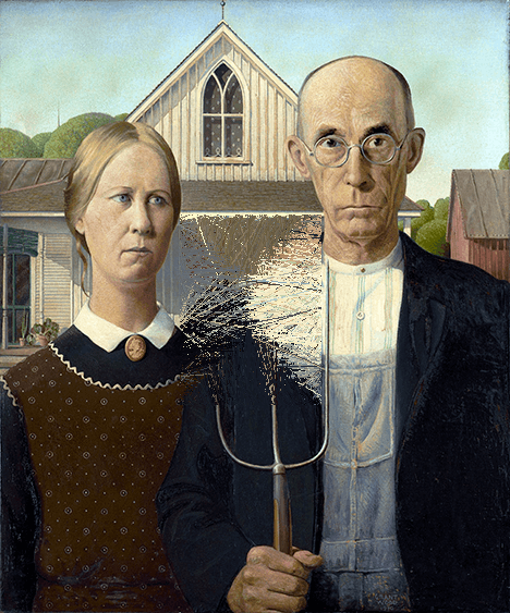
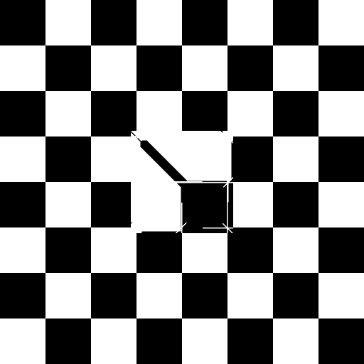
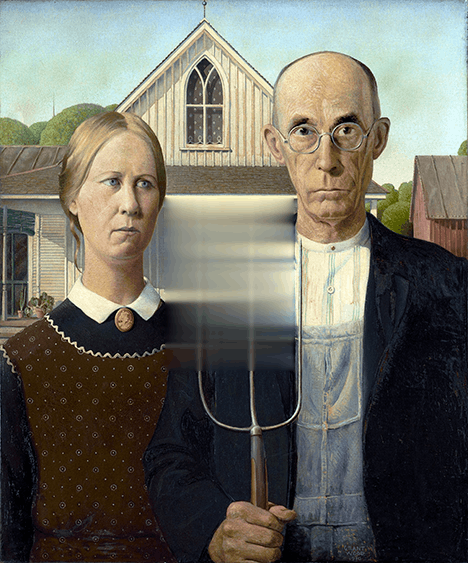
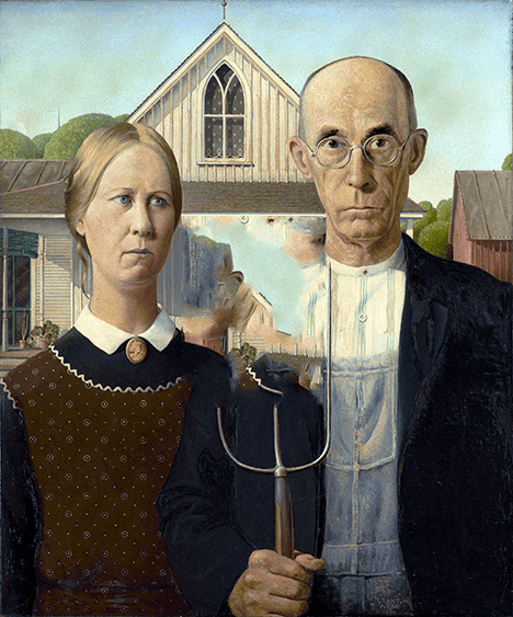
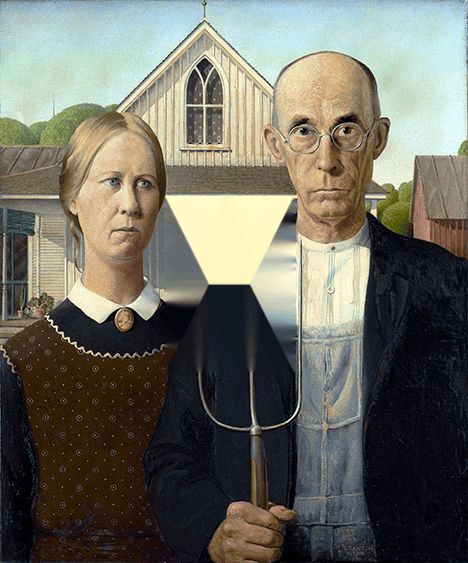
;~ inpaint("gothic_in.png", "gothic_out.png")
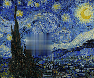
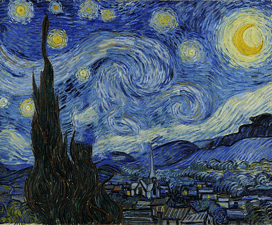
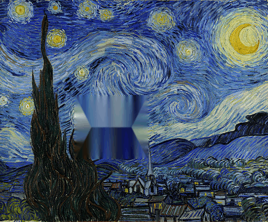
;~ inpaint("starry_in.png", "starry_out.png")
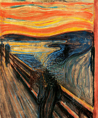
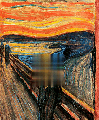
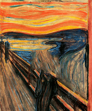
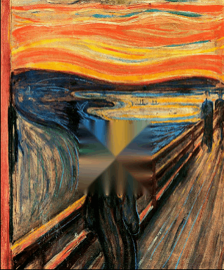
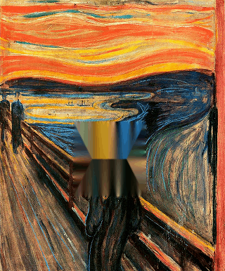
;~ inpaint("scream_in.png", "scream_out.png")
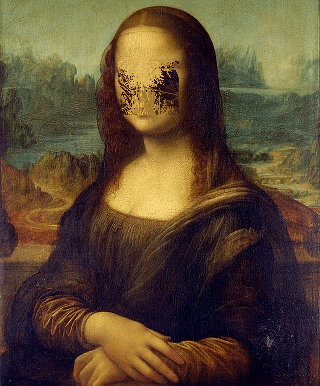
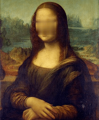
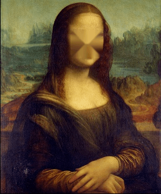
;~ inpaint("mona_in.png", "mona_out.png")
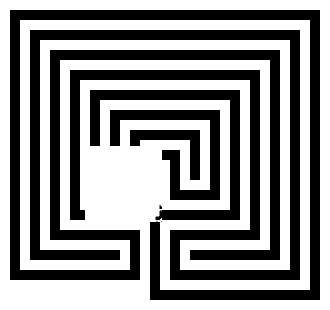
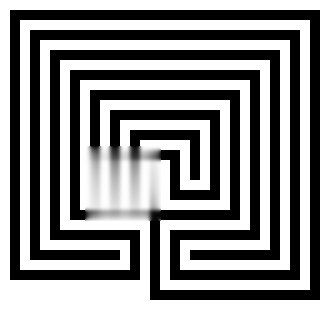
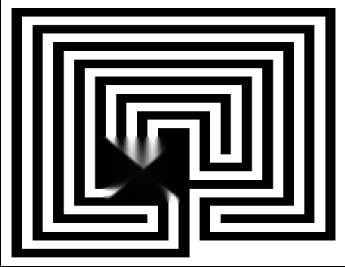
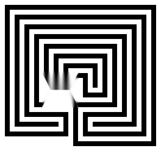
;~ inpaint("maze_in.png", "maze_out.png")
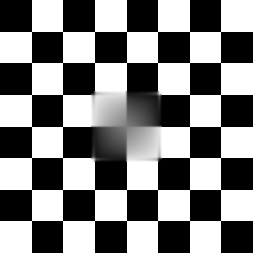
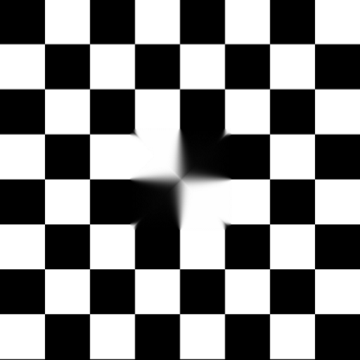
;~ inpaint("checker_in.png", "checker_out.png")
just uncomment the example you want to run using CTRL+Q.
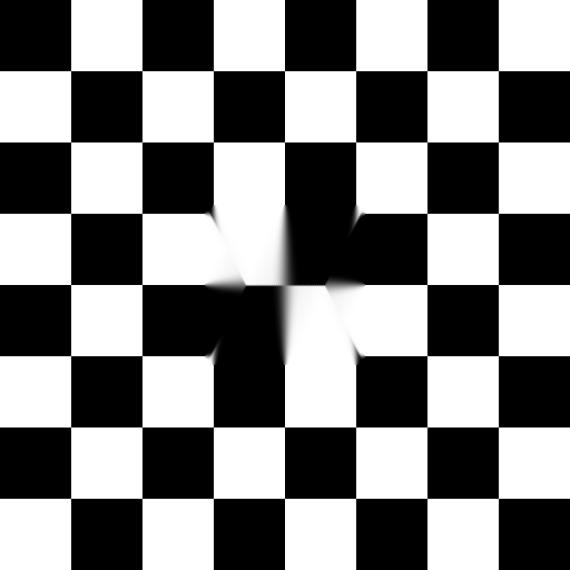
Official Test Files
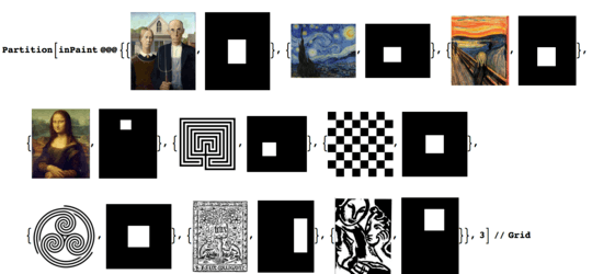
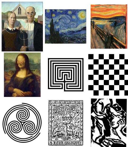
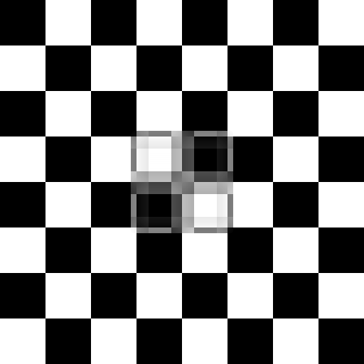
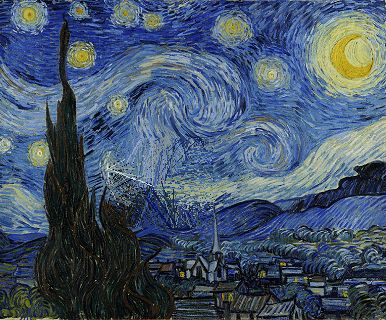
This algorithm is made to be adjusted for each image. Therefore, the default values (and also the default masks) are completely suboptimal. The default values are chosen so that every sample can be processed in a reasonable amount of time. I highly recommend to play with irregularly shaped masks and better window sizes. Click the images to enlarge!
Checkerboard
 →
→ 
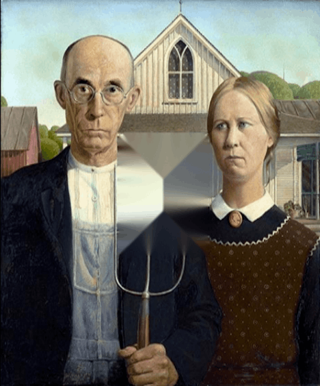
American Gothic
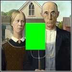 →
→ 
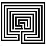
Maze
 →
→ 
Mona Lisa
 →
→ 
(terrible mask)
Scream
 →
→ 
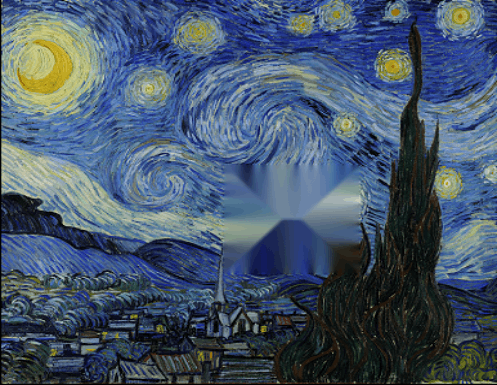
Starry
 →
→ 
Real-World Examples
These all use custom hand-drawn masks.


If you have other interesting images you'd like to see included, leave a comment.
EBII Improvements
There are multiple variants of EBII out there, created by various researchers. AnkurKumar Patel caught my attention with his collection of papers [24] on various EBII improvements.
Specifically the paper "Improved Robust Algorithm For Exemplar Based Image Inpainting" [25] mentions two improvements on the weighing of the priority values.
The improvement
The effective modification is in Step 1 (see above) of the algorithm, and extends the C(p) and D(p) effect on the priority rating for this pixel using this:
In the formula for C and D given above,  and
and  are respectively the normalization factor (e.g., α = 255), the isophote vector, and the unit vector orthogonal to the front
  in the point p.
Further,

The priority function is defined as the weight sum of the regularized confidence term C(p) and the new data term D(p). Where α is the adjustment coefficient, satisfying 0Rp(p) is defined follows:

Where α and β are respectively the component weights of the confidence and the data terms. Note that α+β=1.
Objective scoring
What is really interesting though is that this paper contains a proposed (and simple!) method for scoring the performance if EBII algorithms. Take this with a grain of salt though, as this is a method chosen by the paper authors themselves to verify the effectiveness of the proposed variance approach and the improvement on several images.
The result evaluation is performed by comparing the PSNR (the Peak Signal-to-Noise Ratio [26]) between the restored image and original image. Generally the higher the PSNR value the larger the similarity of the repaired image to the original. The equation to calculate the PSNR is as follows:

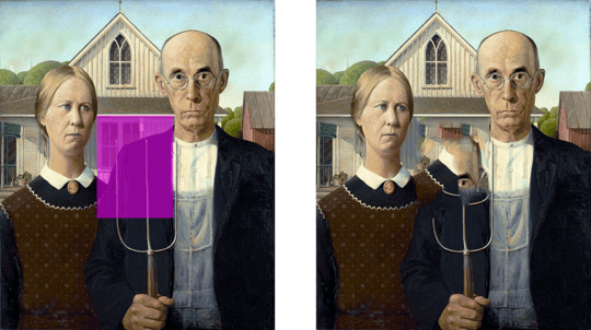
These are the staggering 2 (two!) real-world test images they used:


The conclusion is as disappointing as the quality of the paper itself. It shows very little improvement. The main thing here is a possible object scoring method for this kind of challenge (and other image-repair challenges):
+-------+---------------+----------+
| Image | EBII Original | Improved |
+-------+---------------+----------+
|     1 |       52.9556 |  53.7890 |
|     2 |       53.9098 |  53.8989 |
+-------+---------------+----------+
Meh.
Research to be done
(Specific to EBII)
a) Pre-Processing
Everything comes down to the "Magic Erase" principle that the algorithm should "just work" for everything. My naive solution for this is a color-based amplification (see above), but there are better ways. I'm thinking of recognizing the geometric mean of all traceable texels to auto-adjust the window size and making the stamp size (also my improvement) dependent on texel- and whole-image resolution. Research has to be done here.
b) Post-Processing
The original authors already did a great job of debunking all post processing filters that come in mind. Today, I tried something else, inspired by the always uncanny Mona Lisa (thanks undergroundmonorail). If you take just the inpainted region and apply a new mask to all strange blocks of color and feed that into a despeckling algorithm, you're left with an almost perfect result. I may explore this some time in the future.
[X] — Object Removal by Exemplar-Based Inpainting by A. Criminisi, P. Perez, K. Toyama
[1] — M. Ashikhmin. Synthesizing natural textures. In Proc. ACM Symp. on Interactive 3D Graphics, pp. 217–226, Research Triangle Park, NC, Mar 2001.
[5] — M. Bertalmio, L. Vese, G. Sapiro, and S. Osher. Simultaneous structure and texture image inpainting. to appear, 2002
[6] — R. Bornard, E. Lecan, L. Laborelli, and J-H. Chenot. Missing data correction in still images and image sequences. In ACM Multimedia, France, Dec 2002.
[7] — T. F. Chan and J. Shen. Non-texture inpainting by curvature-driven diffusions (CDD). J. Visual Comm. Image Rep., 4(12), 2001.
[8] — J.S. de Bonet. Multiresolution sampling procedure for analysis and synthesis of texture images. In Proc. ACM Conf. Comp. Graphics (SIGGRAPH), volume 31, pp. 361–368, 1997.
[9] — A. Efros and W.T. Freeman. Image quilting for texture synthesis and transfer. In Proc. ACM Conf. Comp. Graphics (SIGGRAPH), pp. 341–346, Eugene Fiume, Aug 2001.
[10] — A. Efros and T. Leung. Texture synthesis by non-parametric sampling. In Proc. ICCV, pp. 1033–1038, Kerkyra, Greece, Sep 1999.
[11] — W.T. Freeman, E.C. Pasztor, and O.T. Carmichael. Learning low level vision. Int. J. Computer Vision, 40(1):25–47, 2000.
[12] — D. Garber. Computational Models for Texture Analysis and Texture Synthesis. PhD thesis, Univ. of Southern California, USA, 1981.
[13] — P. Harrison. A non-hierarchical procedure for re-synthesis of complex texture. In Proc. Int. Conf. Central Europe Comp. Graphics, Visua. and Comp. Vision, Plzen, Czech Republic, Feb 2001.
[14] — D.J. Heeger and J.R. Bergen. Pyramid-based texture analysis/synthesis. In Proc. ACM Conf. Comp. Graphics (SIGGRAPH), volume 29, pp. 229–233, Los Angeles, CA, 1995.
[15] — A. Hertzmann, C. Jacobs, N. Oliver, B. Curless, and D. Salesin. Image analogies. In Proc. ACM Conf. Comp. Graphics (SIGGRAPH), Eugene Fiume, Aug 2001.
[16] — H. Igehy and L. Pereira. Image replacement through texture synthesis. In Proc. Int. Conf. Image Processing, pp. III:186–190, 1997.
[17] — G. Kanizsa. Organization in Vision. Praeger, New York, 1979.
[19] — L. Liang, C. Liu, Y.-Q. Xu, B. Guo, and H.-Y. Shum. Real-time texture synthesis by patch-based sampling. In ACM Transactions on Graphics, 2001.
[22] — L.-W. Wey and M. Levoy. Fast texture synthesis using tree-structured vector quantization. In Proc. ACM Conf. Comp. Graphics (SIGGRAPH), 2000.
[23] — A. Zalesny, V. Ferrari, G. Caenen, and L. van Gool. Parallel composite texture synthesis. In Texture 2002 workshop - (in conjunction with ECCV02), Copenhagen, Denmark, Jun 2002.
[24] — AkurKumar Patel, Gujarat Technological University, Computer Science and Engineering
[25] — Improved Robust Algorithm For Exemplar Based Image Inpainting
[26] — Wikipedia, Peak-Signal-to-Noise-Ratio




 , where
 , where


 and
and  are respectively the normalization factor (e.g., α = 255), the isophote vector, and the unit vector orthogonal to the front
  in the point p.









1Can we accept the mask input as text arguments (eg.
inpaint.exe left top width height img.jpg)? – mınxomaτ – 2016-01-29T22:21:07.9831Sure, the input/output format is not really that important, as it is a popularity contest where first of all the performance of your algorithm is important. – flawr – 2016-01-29T22:38:46.460
24This is a very practical challenge. It is possible the results will be better than existing algorithms used in GIMP and other open source image editing software. Fortune, Fame, and Glory could be yours! – Sparr – 2016-01-29T23:06:02.713
6@Sparr and finally ugly watermarks can be removed from downloaded media;) – Andras Deak – 2016-01-29T23:07:49.740
Can we have some clarification on whether inpainting builtins are permitted? – trichoplax – 2016-01-30T23:48:08.533
2Builtins are perfectly ok, I do doubt their going to be very popular though. – flawr – 2016-01-30T23:49:09.967
Are masks always guaranteed to be rectangular? If not, can we have some test cases with non-rectangular masks? – SuperJedi224 – 2016-01-31T03:54:25.940
No, the mask is always rectangular as specified. – flawr – 2016-01-31T10:35:09.920