​Plane​ ​Blow​up​

9

1

The Blow-up is a powerful tool in algebraic geometry. It allows the removal of singularities from algebraic sets while preserving the rest of their structure.

If you're not familiar with any of that don't worry, the actual computation is not difficult to understand (see below).

In the following we are considering the blow-up of the point \$(0,0)\$ of an algebraic curve in 2D. An algebraic curve in 2D is given by the zero-locus of a polynomial in two variables (e.g. \$p(x,y) = x^2 + y^2 - 1\$ for the unit circle, or \$p(x,y) = y-x^2\$ for a parabola). The blowup of that curve (in \$(0,0)\$) is given by two polynomials \$r,s\$ as defined below. Both \$r\$ and \$s\$ do describe \$p\$ with the (possible) singularity at \$(0,0)\$ removed.

Challenge

Given some polynomial \$p\$, find \$r\$ and \$s\$ as defined below.

Definition

First of all note that everything I say here is simplified, and does not completely correspond to the actual definitions.

Given a polynomial \$p\$ in two variables \$x,y\$ the blowup is given by two polynomials \$r,s\$ again each in two variables.

To get \$r\$ we first define \$R(x,v) := p(x,vx)\$. Then \$R(x,v)\$ is probably a multiple of \$x\$, i.e. \$R(x,v) = x^n \cdot r(x,v)\$ for some \$n\$ where \$x\$ does not divide \$r(x,v)\$. Then \$r(x,v)\$ is basically what remains after the division.

The other polynomial is defined exactly the same, but we switch the variables: First write \$S(u,y) := p(uy,y)\$. Then \$s\$ is defined such that \$S(u,y) = y^m \cdot s(u,y)\$ for some \$m\$ where \$y\$ does not divide \$s(u,y)\$.

In order to make it clearer consider following

Example

Consider the curve given by the zero locus of \$p(x,y) = y^2 - (1+x) x^2\$. (It has a singularity at \$(0,0)\$ because there is no well defined tangent at that point. )

Then we find

$$R(x,v) = p(x,vx) = v^2x^2-(1+x)x^2 = x^2 (v^2-1-x)$$

Then \$r(x,v) = v^2 -1 -x\$ is the first polynomial.

Similarly

$$S(u,y) = p(uy,y) = y^2 - (1+ uy) u^2 y^2 = y^2 (1 - (1 + uy)u^2)$$

Then \$s(u,y) = 1 - (1 + uy)u^2 = 1 - u^2 + u^3y\$.

rs

Input/Output Format

(Same as here.) The polynomials are represented given as(m+1) x (n+1) matrices/lists of lists of integer coefficients, in the example below the terms of the coefficients are given in their position:

[   1 * 1,   1 * x,   1 * x^2,   1 * x^3,  ... , 1 * x^n ]
[   y * 1,   y * x,   y * x^2,   y * x^4,  ... , y * x^n ]
[   ...  ,   ...   ,   ...   ,    ...   ,  ... ,   ...   ]
[ y^m * 1, y^m * x, y^m * x^2, y^m * x^3 , ..., y^m * x^n]

So an ellipse 0 = x^2 + 2y^2 -1 would be represented as

[[-1, 0, 1],
 [ 0, 0, 0],
 [ 2, 0, 0]]

If you prefer you can also swap x and y. In each direction you are allowed to have trailing zeros (i.e. coefficients of higher degrees that are just zero). If it is more convenient you can also have staggered arrays (instead of a rectangular one) such that all sub sub-arrays contain no trailing zeros.

  • The output format is the same as the input format.

Examples

More to be added (source for more)
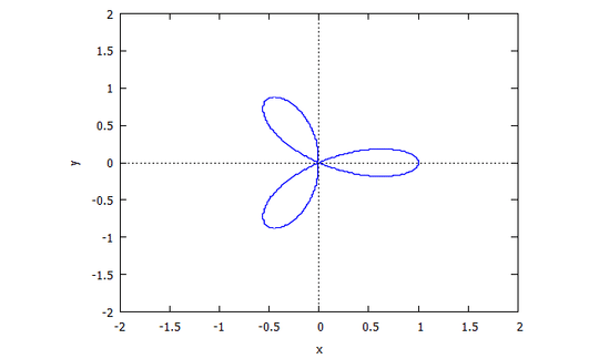
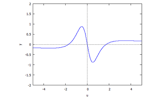
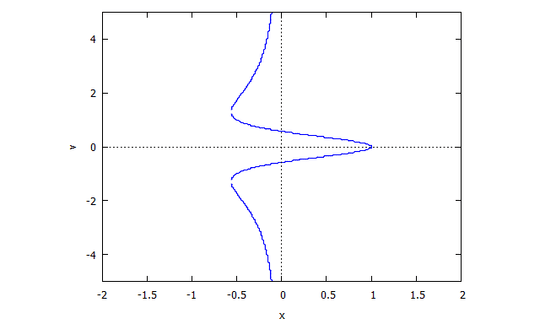
Trifolium
p(x,y) = (x^2 + y^2)^2 - (x^3 - 3xy^2)
r(x,v) = v^4  x + 2  v^2  x + x + 3  v^2 - 1
s(u,y) = u^4  y + 2  u^2  y + y - u^3 + 3  u
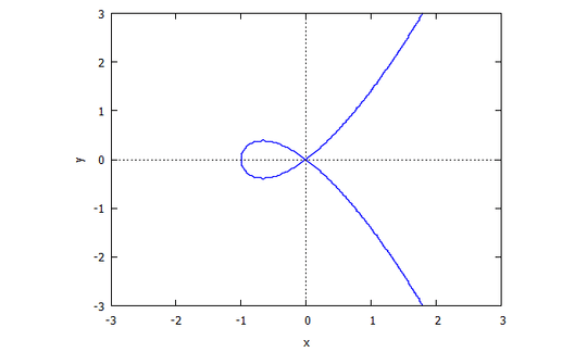
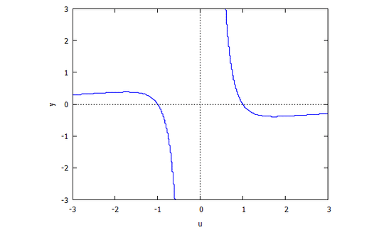
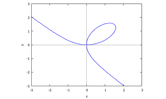
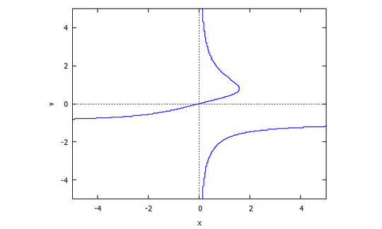
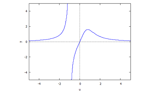
p r s

Descartes Folium
p(x,y) = y^3 - 3xy + x^3
r(x,v) = v^3  x + x - 3v
s(u,y) = u^3  y + y - 3u

p r s

Examples w/o pictures

Trifolium:
p:
[[0,0,0,-1,1],
 [0,0,0, 0,0],
 [0,3,2, 0,0],
 [0,0,0, 0,0],
 [1,0,0, 0,0]]
r: (using the "down" dimension for v instead of y)
[[-1,1],
 [ 0,0],
 [ 3,2],
 [ 0,0],
 [ 0,1]]
s: (using the "right" dimension for u instead of x)
[[0,3,0,-1,0],
 [1,0,2, 0,1]]

Descartes Folium:
p:
[[0, 0,0,1],
 [0,-3,0,0],
 [0, 0,0,0],
 [1, 0,0,0]]
r:
[[ 0,1],
 [-3,0],
 [ 0,0],
 [ 0,1]]
s:
[[0,-3,0,0],
 [1, 0,0,1]]

Lemniscate:
p: 
[[0,0,-1,0,1],
 [0,0, 0,0,0],
 [1,0, 0,0,0]]
r:
[[-1,0,1],
 [ 0,0,0],
 [ 1,0,0]]
s:
[[1,0,-1,0,0],
 [0,0, 0,0,0],
 [0,0, 0,0,1]]

Powers:
p:
[[0,1,1,1,1]]

r:
[[1,1,1,1]]

s:
[[0,1,0,0,0],
 [0,0,1,0,0],
 [0,0,0,1,0],
 [0,0,0,0,1]]

flawr

Posted 2019-08-30T08:59:48.967

Reputation: 40 560

7This title definitely isn't what I thought it was... – negative seven – 2019-08-30T09:46:29.987

Suggested testcase: 0+x+x^2+x^3+x^4 – user41805 – 2019-08-31T14:18:04.013

@Cowsquack Added it! – flawr – 2019-08-31T15:25:07.667

Answers

5

Python 3 + numpy, 165 134 bytes

lambda p:(r(p),r(p.T).T)
from numpy import*
def r(p):w,l=where(p);s=w+l;n=min(s);o=zeros((len(p),max(s)-n+1));o[w,s-n]=p[w,l];return o

Try it online!

The function takes one numpy 2D array p as input and returns a tuple of (r,s) of two numpy 2D arrays.

The breakdown of the solution is as follows. In order to compute the polynomial \$r\$, we rewrite each term \$x^jy^i\$ of \$p\$ into \$x^{j+i}(\frac{y}{x})^i\$, and it becomes \$x^{j+i}u^i\$ in \$p(x,ux)\$. So we can rearrange the input \$(m+1)\times (n+1)\$ matrix \$P\$ into a \$(m+1)\times (m+n-1)\$ matrix \$D\$ corresponding to \$p(x,ux)\$ by setting \$D[i,j+i]=P[i,j]\$. Then we eliminate all-zero columns at the beginning and end of \$D\$ to perform a reduction and get the output matrix \$R\$ for \$r\$.

To compute \$s\$, we simply swap \$x\$ and \$y\$, repeat the same process, and then swap them back. This corresponds to computing \$R\$ for \$P^T\$ and then transposes the outcome.

The following ungolfed code shows the above computation process.

Ungolfed (Basic)

import numpy as np

def r(p):
    num_rows, num_cols = p.shape
    deg_mat = np.zeros((num_rows, num_rows + num_cols - 1))
    for i, row in enumerate(p):
        deg_mat[i, i:i+num_cols] = row
    non_zero_col_idx, = np.where(deg_mat.any(axis=0))
    return deg_mat[:,non_zero_col_idx.min():non_zero_col_idx.max()+1]

def rs(p):
    return r(p), r(p.T).T

Try it online!

A further improvement of the solution computes the matrix \$R\$ in one single pass based on \$R[i,j+i-c]=P[i,j]\$, where \$c=\min_{P[i,j]\neq 0}i+j\$.

Ungolfed (Improved)

import numpy as np

def r(p):
    y_deg, x_deg = np.where(p)  # Retrieve degrees of y and x for non-zero elements in p
    total_deg = y_deg + x_deg
    min_total_deg = total_deg.min()
    max_total_deg = total_deg.max()
    out = np.zeros((p.shape[0], max_total_deg - min_total_deg + 1))
    out[y_deg, y_deg + x_deg - min_total_deg] = p[y_deg, x_deg]
    return out

def rs(p):
    return r(p), r(p.T).T

Try it online!

Joel

Posted 2019-08-30T08:59:48.967

Reputation: 1 691

3

APL (Dyalog Unicode), 38 37 bytes

1 byte saved thanks to ngn by using +/∘⍴ in place of the dummy literal 0

⊢∘⍉\+/∘⍴{q↓⍨⊃⍸×∨/q←(-⍳≢⍉⍵)⊖⍺↑⍵}¨⊂,⊂∘⍉

Try it online!

(a train with ⎕io (index origin) set as 0)

enclosed right argument

, concatenated with

  • ⊂∘ enclosed

  • transposed right argument

\$s\$ is computed from the former, \$r\$ from the latter

¨ on each

+/∘⍴{ ... } perform the following function with left argument

  • +/ sum

      • the shape of the right argument, i.e. get rows+columns

and the right argument will be each of the enclosed matrices.

⍺↑⍵ and take left argument many rows from the right argument , if is deficient in rows (which it will be because rows+columns > rows), it is padded with enough 0s

The computation of substituting \$vx\$ or \$uy\$ in place of \$y\$ or \$x\$ is done by rotating the columns of by their index, and since is padded with 0s, columns of are effectively prepended by the desired amount of 0s.

rotate columns by

  • ⍉⍵ transposed

  • count rows, all together, ≢⍉⍵ gets the number of columns in

  • range 0 .. count-1

  • - negated, to rotate in the other direction and the default for , to ultimately yield 0 ¯1 ¯2 ... -(count-1), this automatically vectorises across each column such that the 0-th column is rotated by 0, the 1-st by 1, ...

q← assign this to variable q

Now to divide the polynomial by the largest power of \$x\$ or \$y\$, the leading all-0 rows have to be removed.

∨/ reduce by LCM across each row, if the row is all-0s, this yields 0, otherwise it gives a positive number

× get its sign, 00 and positive number → 1

indices of truthies, i.e. indices of 1s

pick the first element, ⊃⍸ simply gets the index of the first 1

q↓⍨ drops that many rows from q, again ⎕io←0 helps in returning the correct value for dropping the leading all-0 rows

(exit function)

\$s\$ is already achieved, to get \$r\$ the second value has to be transposed via ⊢∘⍉\


Other approaches are listed below.

⍝(⊢∘⍉\+/∘⍴{q↓⍨⊃⍸×∨/q←(-⍳≢⍉⍵)⊖⍺↑⍵}¨⊂,⊂∘⍉)¨a
⍝(⊢∘⍉\∘⌽⍴{q↓⍨⊃⍸×∨/q←(-⍳⍺)⊖⍵↑⍨+/⍴⍵}¨⊂∘⍉,⊂)¨a
⍝(⊢∘⍉\⌽∘⍴{q↓⍨⊃⍸×∨/q←(-⍳⍺)⊖⍵↑⍨+/⍴⍵}¨⊂,⊂∘⍉)¨a
⍝(⊢∘⍉\0{q↓⍨⊃⍸×∨/q←(-⍳≢⍉⍵)⊖⍵↑⍨+/⍴⍵}¨⊂,⊂∘⍉)¨a
⍝(⊢∘⍉\+/∘⍴({⍵↓⍨⊃⍸×∨/⍵}(-∘⍳1⊃⊢∘⍴)⊖↑)¨⊂,⊂∘⍉)¨a
⍝(⊂∘⍉∘⊃@0⍴{q↓⍨⊃⍸×∨/q←(-⍳⍺)⊖⍵↑⍨+/⍴⍵}¨⊂∘⍉,⊂)¨a
⍝{⊢∘⍉\{q↓⍨⊃⍸×∨/q←(-⍳≢⍉⍵)⊖⍵↑⍨+/⍴⍵}¨⍵(⍉⍵)}¨a
⍝(⊢∘⍉\(({⍵↓⍨⊃⍸×∨/⍵}(-∘⍳1⊃⍴)⊖⊢↑⍨1⊥⍴)¨⊂,⊂∘⍉))¨a
⍝(0 1{⍉⍣⍺⊢q↓⍨⊃⍸×∨/q←(-⍳≢⍉⍵)⊖⍵↑⍨+/⍴⍵}¨⊂,⊂∘⍉)¨a
⍝{⊢∘⍉\{q[;⍸×∨\∨⌿q←↑(,\0⍴⍨≢⍵),¨↓⍵]}¨⍵(⍉⍵)}¨a
⍝{⊢∘⍉\{q↓⍨1⍳⍨×∨/q←(-⍳≢⍉⍵)⊖⍵↑⍨+/⍴⍵}¨⍵(⍉⍵)}¨a
⍝(⊢∘⍉\(((⊢↓⍨1⍳⍨0≠∨/)(-∘⍳1⊃⍴)⊖⊢↑⍨1⊥⍴)¨⊂,⊂∘⍉))¨a
⍝{⊢∘⍉\{q[⍸×∨\∨/q←(-⍳≢⍉⍵)⊖⍵↑⍨+/⍴⍵;]}¨⍵(⍉⍵)}¨a
⍝{⊢∘⍉\{q↓⍨+/0=∨\∨/q←(-⍳≢⍉⍵)⊖⍵↑⍨+/⍴⍵}¨⍵(⍉⍵)}¨a
⍝{⊢∘⍉\{q↓⍨⌊/+⌿∧⍀0=q←(-⍳≢⍉⍵)⊖⍵↑⍨+/⍴⍵}¨⍵(⍉⍵)}¨a
⍝(⌽∘⍉¨1↓({⊖⍉q[⍸×∨\∨/q←(-⍳≢⍉⍵)⊖⍵↑⍨+/⍴⍵;]}\3/⊂))¨a
⍝{⊢∘⍉\{↑(↓q)/⍨∨\×∨/q←(-⍳≢⍉⍵)⊖⍵↑⍨+/⍴⍵}¨⍵(⍉⍵)}¨a
⍝f←⊢∘⍉\⋄{f{q[⍸×∨\∨/q←(-⍳≢⍉⍵)⊖⍵↑⍨+/⍴⍵;]}¨f⍵⍵}¨a
⍝{1↓⌽∘⍉¨{⊖⍉q[⍸×∨\∨/q←(-⍳≢⍉⍵)⊖⍵↑⍨+/⍴⍵;]}\3/⊂⍵}¨a
⍝{f←{q[⍸×∨\∨/q←(-⍳≢⍉⍵)⊖⍵↑⍨+/⍴⍵;]}⋄(f⍵)(⍉f⍉⍵)}¨a
⍝{⊢∘⍉\{↑(↓q)/⍨∨\0≠∨/q←(-⍳≢⍉⍵)⊖⍵↑⍨+/⍴⍵}¨⍵(⍉⍵)}¨a
⍝{⊢∘⍉\{(0~⍨∊⍵)@(↓⍉(⊢-⌊/)@1+⍀⍉↑⍸0≠⍵)⊢0⍴⍨,⍨⌈/⍴⍵}¨⍵(⍉⍵)}¨a

user41805

Posted 2019-08-30T08:59:48.967

Reputation: 16 320